Wine Map - 03: Solar Radiation Data

Solar Data

In Part 01 of this series, Andrew Durkan identified that vines need around 1300 hours of sunshine, and as such, sunlight was going to be a significant factor. After some searching for sources, I settled on the outputs from the Global Solar Atlas. This resource doesn’t provide sunlight hours but instead has other measures, including:

Specific photovoltaic power output
Direct normal irradiation
Global horizontal irradiation
Diffuse horizontal irradiation
Global irradiation for optimally tilted surface

I figured that this dataset — whilst not exactly what I was after — should be a strong covariant. I downloaded the Annual and monthly statistics where available.

pacman::p_load(tidyverse, curl, sf, glue)

#https://globalsolaratlas.info/download/australia
root = "input/05 solar"
file_name = "Australia_GISdata_LTAy_YearlyMonthlyTotals_GlobalSolarAtlas-v2_GEOTIFF"

zip_url = glue("https://api.globalsolaratlas.info/download/Australia/{file_name}.zip")
zip_path = glue("{root}/{file_name}.zip")

curl_download(zip_url, zip_path)
zip::unzip(zip_path, exdir = glue("{root}"))

The zip file unpacked into the following file structure:

├─── 05 solar │ ├─── Australia_GISdata_LTAy_YearlyMonthlyTotals_GlobalSolarAtlas-v2_GEOTIFF │ │ └─── monthly

This data was in EPSG:4326 (WGS 84) at various resolutions, specifically:

Solar resource data (GHI, DIF, GTI, DNI): 9 arcsecs ~ 250 m
Specific Photovoltaic Power Output: 30 arcsecs ~ 1 km
Optimal Tilt Angle: 120 arcsec ~ 4 km
The project so had a spatial resolution of 150 arcsecs ~ 4.6km, as determined by using the formulas below (Nominals radius of Earth at the equator of 6371 km).

\[d = R\theta\] \[d = \left(360 \over 8640\right) \times \left( \pi \over 180\right) \times 6371 km\]

Some interpolation will be required to compare these data sets directly. $GDAL$, ever faithful, has this functionality in the $translate$ function. From the documentation, I need to pass the $-tr$ option and the x and y resolutions in addition to the source and destination file paths.
The sf package has a handy helper function wrapped around $GDAL$’s native utilities sf::gdal_utils which will be the basis of the function I will map over the GeoTIFF files.

On inspection, however, I noticed a second issues:

> raster::raster("input/05 solar/Australia_GISdata_LTAy_YearlyMonthlyTotals_GlobalSolarAtlas-v2_GEOTIFF/DIF.tif" )
class      : RasterLayer 
dimensions : 14000, 19200, 268800000  (nrow, ncol, ncell)
resolution : 0.0025, 0.0025  (x, y)
extent     : 112, 160, -44, -9  (xmin, xmax, ymin, ymax)
crs        : +proj=longlat +datum=WGS84 +no_defs +ellps=WGS84 +towgs84=0,0,0 
source     : C:/Users/Mathew Merryweather/Documents/GitHub/wine_map/input/05 solar/Australia_GISdata_LTAy_YearlyMonthlyTotals_GlobalSolarAtlas-v2_GEOTIFF/DIF.tif 
names      : DIF 
values     : 383.147, 916.412  (min, max)

Take a look at the extent compared to my projects:

"Source Raster"
extent     : 112, 160, -44, -9  (xmin, xmax, ymin, ymax)

"Project"
extent     : 112, 154, -44, -10  (xmin, xmax, ymin, ymax)

I need to “crop” into the project and modify the extent as well. I used sf::gdal_utils again but this time passing the $-projwin$ arguments and my extent coordinates. Due to limitations under the hood, I couldn’t pipe the results from one call into the destination of another which would have been much more elegant. Instead, I dropped the first call to a TEMP file then input that into the second call. I wrapped both of these calls into a function for mapping.

gdal_resize = function(source, destination, res){
  # https://gdal.org/programs/gdal_translate.html
  # gdal_translate -tr 0.1 0.1 "C:\dem.tif" "C:\dem_0.1.tif"
  sf::gdal_utils("translate",
                 source = source,
                 destination = str_replace(destination, "\\.tif","\\_temp\\.tif"),
                 options = c("-tr", res, res))
  # gdal_translate -projwin ulx uly lrx lry inraster.tif outraster.tif`
  sf::gdal_utils("translate",
                 source = str_replace(destination, "\\.tif","\\_temp\\.tif"),
                 destination = destination,
                 options = c("-projwin",
                             112,
                             -10,
                             154,
                             -44))
  file.remove(str_replace(destination, "\\.tif","\\_temp\\.tif"))

  destination
}

I pilfered the raster to dataframe code from part #2; however, I simplified it for the single-band raster case.

singleband_raster_to_dataframe = function(img){
  img_brick = img %>%
    raster::raster() %>%
    raster::brick()

  col_name = img_brick@data@names[1]

  img_brick@data@values %>%
    as.data.frame() %>%
    set_names(nm = str_to_lower(col_name))
}

I wanted the code to be flexible enough to handle the monthly and annual case with minimal rewriting, so I included a directory check and creation step in the per folder function, leading to the following structure:

├─── 05 solar │ ├─── Australia_GISdata_LTAy_YearlyMonthlyTotals_GlobalSolarAtlas-v2_GEOTIFF │ │ └─── monthly │ └─── scaled │ ├─── annual │ └─── monthly

Additionally, the names (GHI, DIF, DNI) are not very friendly, and I’ll forget what they mean when I get to the modelling steps. To get around this, I also included a named replacement list for the destination files.

folder_of_tifs_to_df = function(input_folder, output_folder){
# Remove the TEMP Variable
input_folder %>% list.files(full.names = T, pattern = "TEMP") %>% file.remove()

files = input_folder  %>%
  list.files(pattern = "tif$",
             full.names = T) %>%
  sort()


if(!dir.exists(output_folder)){
  dir.create(output_folder, showWarnings = F, recursive = T)
}

expand_names = c("PVOUT" = "photovoltaic_power_potential",
                 "GHI" = "global_horizontal_irradiation",
                 "DIF" = "diffuse_horizontal_irradiation",
                 "GTI" = "global_irradiation_for_optimally_tilted_surface",
                 "DNI" = "direct_normal_irradiation",
                 "OPTA" = "optimum_tilt_to_maximize_yearly_yield")

dest_files = input_folder %>%
  list.files(pattern = "tif$") %>%
  sort() %>%
  str_c(output_folder,"/",.) %>%
  str_replace_all(expand_names)

res = 360 / 8640

gdal_resize = function(source, destination, res){
  # https://gdal.org/programs/gdal_translate.html
  # gdal_translate -tr 0.1 0.1 "C:\dem.tif" "C:\dem_0.1.tif"
  sf::gdal_utils("translate",
                 source = source,
                 destination = str_replace(destination, "\\.tif","\\_temp\\.tif"),
                 options = c("-tr", res, res))
  # gdal_translate -projwin ulx uly lrx lry inraster.tif outraster.tif`
  sf::gdal_utils("translate",
                 source = str_replace(destination, "\\.tif","\\_temp\\.tif"),
                 destination = destination,
                 options = c("-projwin",
                             112,
                             -10,
                             154,
                             -44))
  file.remove(str_replace(destination, "\\.tif","\\_temp\\.tif"))

  destination
}
singleband_raster_to_dataframe = function(img){
  img_brick = img %>%
    raster::raster() %>%
    raster::brick()

  col_name = img_brick@data@names[1]

  img_brick@data@values %>%
    as.data.frame() %>%
    set_names(nm = str_to_lower(col_name))
}

df = files %>%
  map2_chr(.y = dest_files,
        .f = gdal_resize,
        res = res) %>%
  map_dfc(singleband_raster_to_dataframe)
df
}

It was now a straightforward exercise to call the folder_of_tifs_to_df function for the annual and monthly cases, then bind the columns into a data frame.

annual_input = glue("{root}/{file_name}")
annual_output = glue("{root}/scaled/annual")
monthly_input = glue("{root}/{file_name}/monthly")
monthly_output = glue("{root}/scaled/monthly")

df_monthly = folder_of_tifs_to_df(monthly_input, monthly_output)
df_annual  = folder_of_tifs_to_df(annual_input, annual_output)

df_points = list(
  lon = seq(from  = 112,
            to    = 154 - res,
            by    = res),
  lat = seq(from  = -44,
            to    = -10 - res,
            by    = res)) %>%
  cross_df() %>%
  arrange(desc(lat), lon)

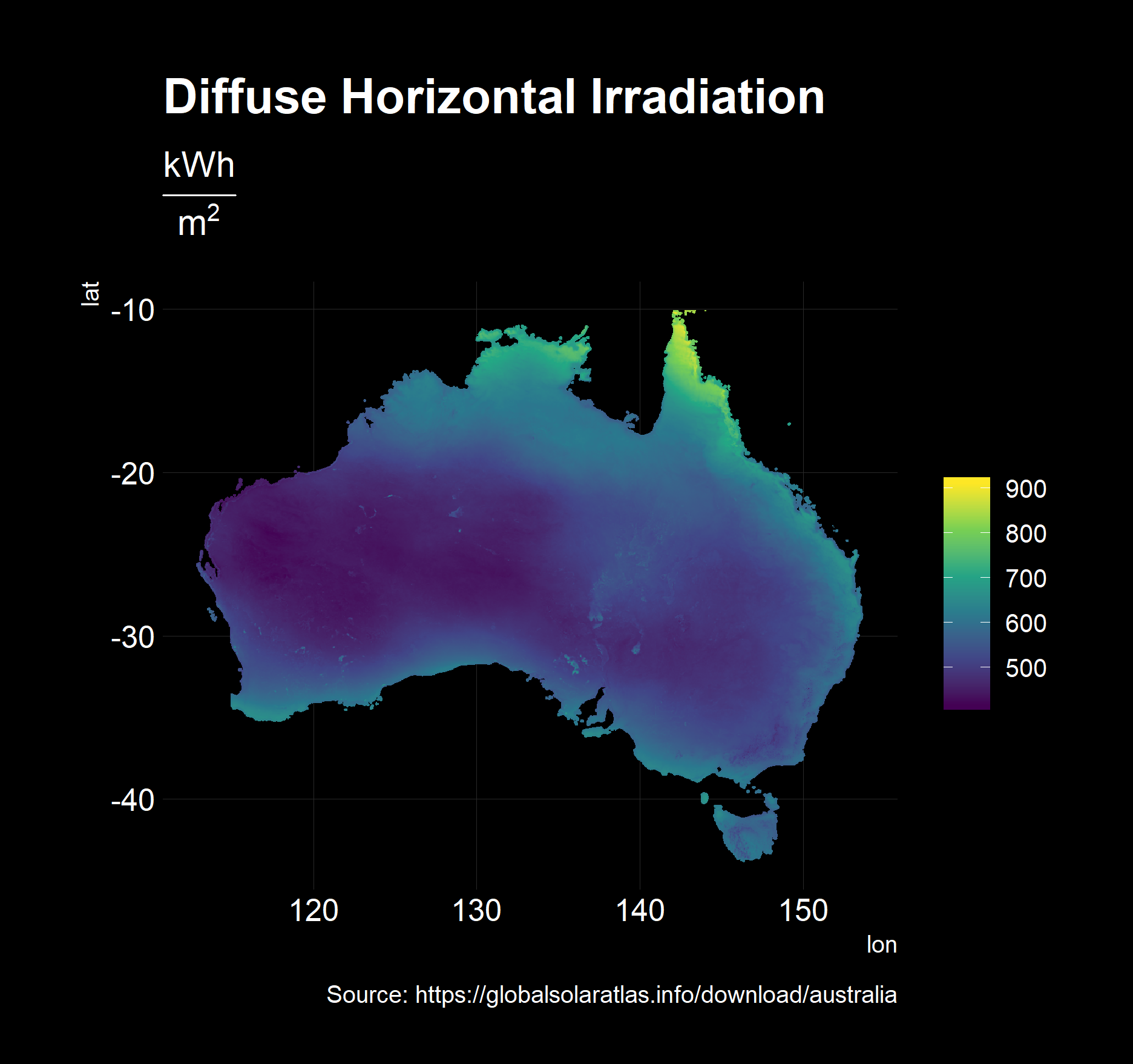
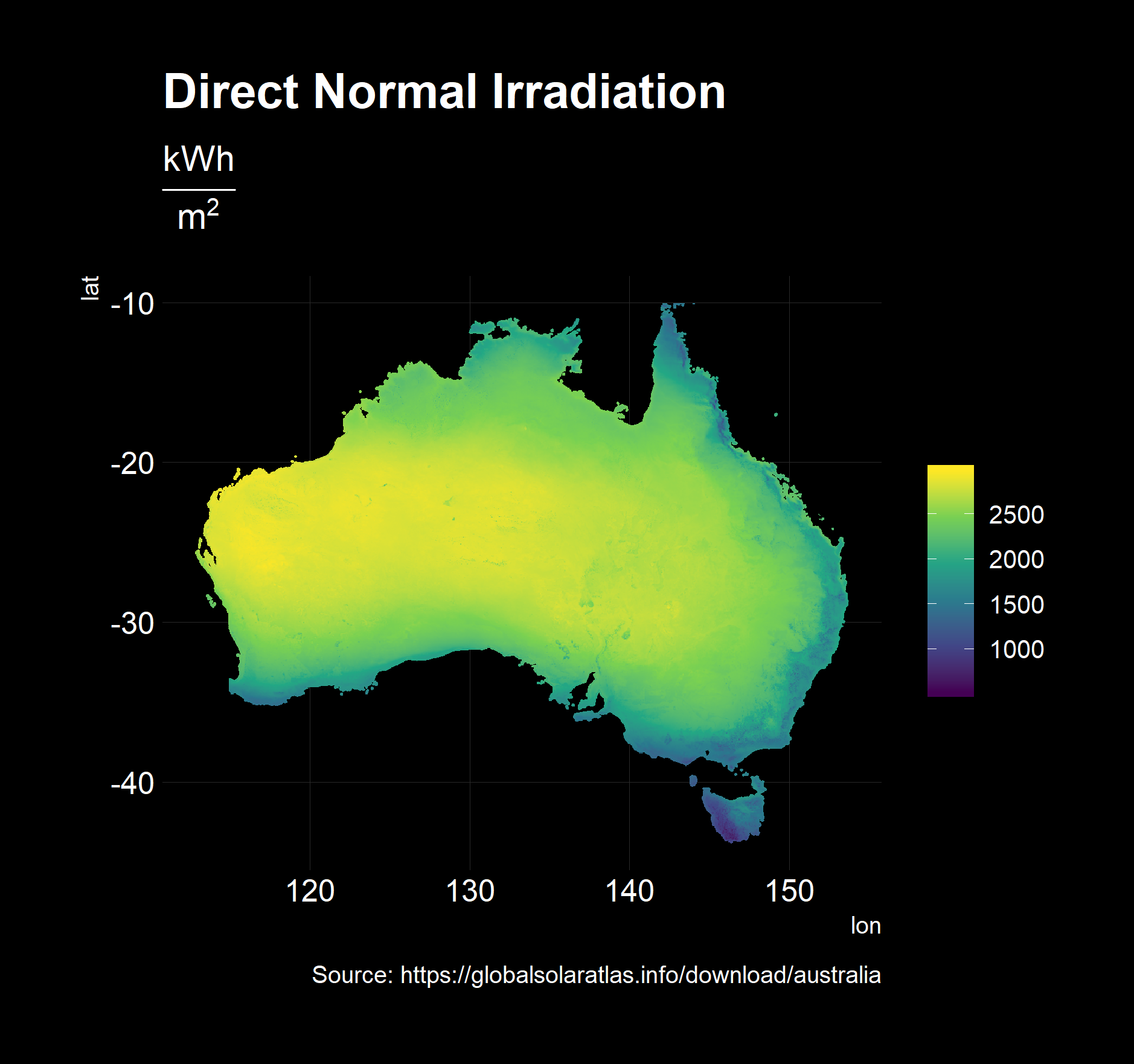
df = df_points %>% bind_cols(df_annual, df_monthly)
df %>% data.table::fwrite(glue("{root}/df_solar.csv"))

For validation, I generated plots of Diffuse Horizontal Irradiation and Direct Normal Irradiation, which appear to have worked correctly.

Diffuse Horizontal Irradiation
Direct Normal Irradiation

The final folder structure is below:
C:. │ Australia_GISdata_LTAy_YearlyMonthlyTotals_GlobalSolarAtlas-v2_GEOTIFF.zip │ df_solar.csv │ ├─── Australia_GISdata_LTAy_YearlyMonthlyTotals_GlobalSolarAtlas-v2_GEOTIFF │ │ DIF.tif │ │ DNI.tif │ │ GHI.tif │ │ GTI.tif │ │ OPTA.tif │ │ PVOUT.tif │ │ │ └─── monthly │ PVOUT_01.tif │ PVOUT_02.tif │ PVOUT_03.tif │ PVOUT_04.tif │ PVOUT_05.tif │ PVOUT_06.tif │ PVOUT_07.tif │ PVOUT_08.tif │ PVOUT_09.tif │ PVOUT_10.tif │ PVOUT_11.tif │ PVOUT_12.tif │ └─── scaled ├─── annual │ diffuse_horizontal_irradiation.tif │ direct_normal_irradiation.tif │ global_horizontal_irradiation.tif │ global_irradiation_for_optimally_tilted_surface.tif │ optimum_tilt_to_maximize_yearly_yield.tif │ photovoltaic_power_potential.tif │ └─── monthly photovoltaic_power_potential_01.tif photovoltaic_power_potential_02.tif photovoltaic_power_potential_03.tif photovoltaic_power_potential_04.tif photovoltaic_power_potential_05.tif photovoltaic_power_potential_06.tif photovoltaic_power_potential_07.tif photovoltaic_power_potential_08.tif photovoltaic_power_potential_09.tif photovoltaic_power_potential_10.tif photovoltaic_power_potential_11.tif photovoltaic_power_potential_12.tif