Part 01

Wine Map Part 2: Geospatial Data

Originally when I planned this post, I was going to walk through QGIS and the nightmare experience I originally had developing this project. The post was to be replete with esoteric $GDAL$ incantations, annotated screenshots and obscure python flotsam, jetsam and errata however that was going to test a self-imposed rule for this website;
All examples must be fully reproducible, with the minimum of human intervation.
In keeping with this principle, I am pleased to say that this time around, the outcomes are higher quality, reproducible and entirely driven from $R$. A much better result.
To achieve this, I had to make heavy use of the $sf$ and $raster$ packages and the Simple Features reference guide.

Geological Data

From Part 1, Jaxon informed me that I would need to take into account the regional geological conditions for the soil component of quantifying terroir.
The data structure I want for my regression model is a wide format, with a single row for each observation (a pixel at a lat/lon coordinate) and columns for each attribute. I want to be able to quantify the impact of each variable, so I want the columns to have 1, for an attribute at that pixel, 0 if not and NA for missing data.

Geoscience Australia has some excellent resources, and I quickly found the dataset I needed: Surface Geology of Australia 1:2.5 million scale dataset 2012 edition. Almost perfect, except that $SHP$ files are represented as rows of polygons in $sf$. Thus, I need to:

Extract each feature individually to a separate layer
Set the layer values to 1 for present
Rasterize that layer into a grid then pivot to a long format
Aggregate the results for each column into a wide dataframe

I downloaded the zip archive using $curl$ and extracted the files associated with the “GeologicUnitPolygons2_5M.shp” layer.

pacman::p_load(tidyverse, curl, sf, glue, fasterize)
zip_url = "https://d28rz98at9flks.cloudfront.net/73140/73140_2_5M_shapefiles.zip"
zip_path = "input/04 geological/classification/73140_2_5M_shapefiles.zip"

curl_download(zip_url, zip_path)

# Unzip all of the 2.5M GeologicUnitPolygon files
zip_files = zip::zip_list(zip_path) %>%
  data.frame() %>%
  filter(str_detect(filename, "GeologicUnitPolygons2_5M")) %>%
  pluck("filename")

zip::unzip(zip_path,
           files = zip_files,
           exdir = "input/04 geological/classification")

The $sf$ package really does make working with geospatial files in $R$ a breeze. You get full access to the $dplyr$ verbs, and polygons are stored in lists inside the $geometry$ column of a data frame.
Due to this, I could import my $SHP$ file with a SQL query, set the CRS to EPSG: 4283 and pipe the result to a transmute for combined subsetting and transformation in four distinct pipe operations.

# Extract the SHP Paths
shp = "input/04 geological/classification/shapefiles" %>%
  list.files(pattern = "shp$",
             full.names = TRUE)

# https://epsg.io/4283
shp_geo = sf::st_read(shp,
                      query = "SELECT * FROM \"GeologicUnitPolygons2_5M\"") %>%
  st_set_crs(NA) %>%
  st_set_crs(4283) %>%
  transmute(FEATUREID,
            STRATNO,
            MAPSYMBOL,
            PLOTSYMBOL,
            NAME = str_remove_all(NAME, " \\d+"),
            DESCR = str_extract(DESCR, "^.*?(?=(;|\\.|\\n))") %>% str_remove_all("(,|\\/)"),
            REPAGE_URI = str_remove(REPAGE_URI, "http://resource.geosciml.org/classifier/ics/ischart/"),
            YNGAGE_URI = str_remove(YNGAGE_URI, "http://resource.geosciml.org/classifier/ics/ischart/"),
            LITHOLOGY = str_replace(LITHOLOGY,";"," and"),
            REPLITH_UR = str_remove(REPLITH_UR,"http://resource.geosciml.org/classifier/cgi/lithology/")
  )

Reading layer `GeologicUnitPolygons2_5M' from data source `C:\Users\Mathew Merryweather\Documents\GitHub\wine_map\input\04 geological\classification\shapefiles\GeologicUnitPolygons2_5M.shp' using driver `ESRI Shapefile'
Simple feature collection with 8343 features and 1 field
geometry type:  POLYGON
dimension:      XY
bbox:           xmin: 112.9125 ymin: -43.64248 xmax: 153.6403 ymax: -10.01599
epsg (SRID):    NA
proj4string:    +proj=longlat +ellps=GRS80 +no_defs

I now had a $sf$ dataframe with the structure below. From here, the approach becomes apparent, for each target column, break out each level into a layer and rasterize.

> glimpse(shp_geo)
Observations: 8,343
Variables: 11
$ FEATUREID  <fct> GA_GUP2.5M_0000001, GA_GUP2.5M_0000002, GA_GUP2.5M_0000003, GA_GUP2.5M_0000004, GA_GUP2.5M_0…
$ STRATNO    <int> 76542, 76542, 76533, 76533, 76542, 76526, 76532, 76526, 76537, 76542, 76542, 76542, 76542, 7…
$ MAPSYMBOL  <fct> Cze, Cze, CPg, CPg, Cze, Cg, CPf, Cg, Cv, Cze, Cze, Cze, Cze, CPf, CPg, Cze, CPg, CPf, CPf, …
$ PLOTSYMBOL <fct> Czu, Czu, CPg, CPg, Czu, Cg, CP, Cg, Cv, Czu, Czu, Czu, Czu, CP, CPg, Czu, CPg, CP, CP, CP, …
$ NAME       <chr> "Cenozoic regolith", "Cenozoic regolith", "Carboniferous to Permian granites", "Carboniferou…
$ DESCR      <chr> "Surficial or regolith units", "Surficial or regolith units", "Mainly felsic intrusive rocks…
$ REPAGE_URI <chr> "Cenozoic", "Cenozoic", "Carboniferous", "Carboniferous", "Cenozoic", "Carboniferous", "Carb…
$ YNGAGE_URI <chr> "Holocene", "Holocene", "Cisuralian", "Cisuralian", "Holocene", "Gzhelian", "Cisuralian", "G…
$ LITHOLOGY  <chr> "regolith", "regolith", "igneous felsic intrusive", "igneous felsic intrusive", "regolith", …
$ REPLITH_UR <chr> "material_formed_in_surficial_environment", "material_formed_in_surficial_environment", "gra…
$ geometry   <POLYGON [°]> POLYGON ((142.8685 -10.0340..., POLYGON ((143.4734 -10.0304..., POLYGON ((142.1909 -…

The function “per_level”, below, uses tidyselect notation to accept a level of a factor, passed as a quoted string and turn it into a symbolic variable ($rlang::sym$). I also use $glue::glue$ extensively to avoid nested $paste0$ calls. I use the “fasterize” package to turn a $sf$ object into a $raster$ however the output is a S$ type object so it doesn’t play nice with the pipe operator (yet).
To subset these objects, use “@” instead of “$”.
I then have a nice, vector of values to turn into a dataframe, set as a data.table (in place in memory) and assign a meaningful name.

per_level = function(level, category){
message(glue("     {str_pad(category,10,'left')} - {level}"))
  sym_level = rlang::sym(level)
  sym_category = rlang::sym(category)
  folder_path = here::here(glue("input/04 geological/features/{category}"))
  file_name = glue::glue("{folder_path}/{category}_{sym_level}.csv")

  shp_subset = shp_geo %>%
    filter(!!sym_category == sym_level) %>%
    mutate(present = 1)

  blank_raster = raster::raster(ncol = 1008,
                                nrow = 816,
                                crs = 4283,
                                xmn = 112,
                                xmx = 154,
                                ymn = -44,
                                ymx = -10,
                                vals = 0)
  ## .@ subsets into S4 objects, could user pipeR but not a fan
  df_raster  = fasterize::fasterize(shp_subset, blank_raster) %>%
    .@data %>%
    .@values %>%
    as.data.frame(row.names = row.names(.)) %>%
    data.table::setDT() %>%
    set_names(str_to_lower(names(.))) %>%
    set_names(nm = glue::glue("{category}_{sym_level}"))

  df_raster %>% data.table::fwrite(file_name)
  df_raster
}

The per category function takes a column from “shp_geo” and maps “per_level” to each level of the column before column binding the results together into a wide dataframe, which is written to an intermediate folder.

per_category = function(category){
  folder_path = here::here(glue("input/04 geological/features/{category}"))
  if(!dir.exists(folder_path)){
    dir.create(folder_path, showWarnings = F, recursive = T)
  }
  message(glue("starting: {category}"))
  #Iterate Per Level
  df_category = shp_geo %>%
    pluck(category) %>%
    unique() %>%
    sort() %>%
    map_dfc(per_level, category)

  df_points %>%
    bind_cols(df_category) %>%
    data.table::fwrite(glue::glue("input/04 geological/features/{category}.csv"))
  df_category
}

Finally, I apply the “per_category” function to a subset of columns and column bind them to a lat/lon data.frame to provide context.
Results are then saved in the top level folder for geological data.

column_levels = df_geo_join %>% select(-(FEATUREID:NAME)) %>%
  as.list() %>%
  map(unique)

res = 360 / 8640
df_points = list(
  lon = seq(from  = 112,
            to    = 154 - res,
            by    = res),
  lat = seq(from  = -44,
            to    = -10 - res,
            by    = res)) %>%
  cross_df() %>%
  arrange(desc(lat), lon)

df_all_geo = df_geo_join %>%
  select(-(FEATUREID:NAME)) %>%
  colnames() %>%
  map_dfc(per_category)

df_points %>%
  bind_cols(df_all_geo) %>%
  data.table::fwrite("input/04 geological/df_all_geo.csv")

Results

I used a helper plotting function to see if the results are correct.

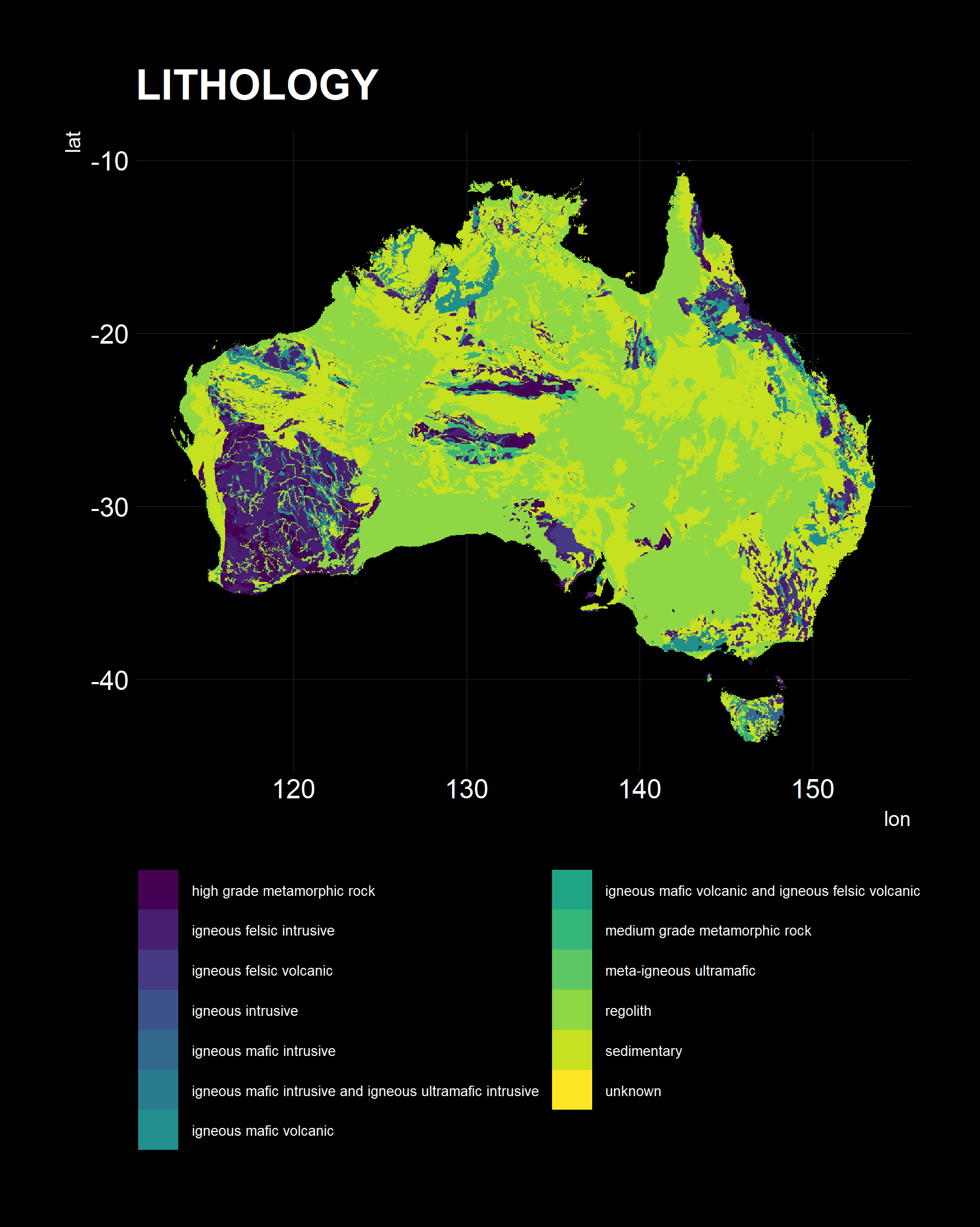
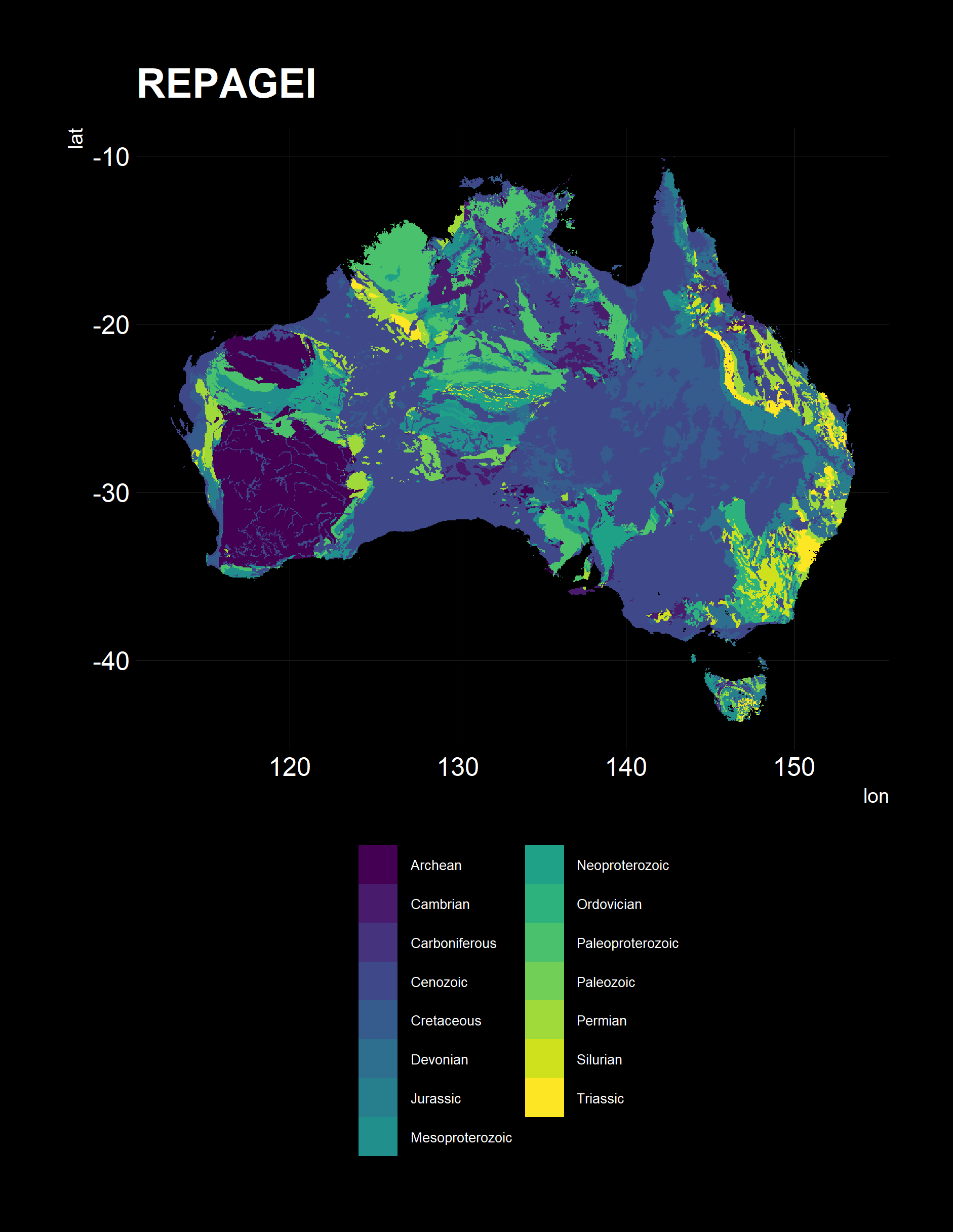
Pleasingly, all have the right orientation, shape and coverage. All three present different pieces of information, of note, is the Lithology, typically sedimentary, metamorphic and granitoid in our wine growing regions, as expected.