Wine Map Part 1: Downloading and manipulating climate data
I was reading a second-hand book I picked up called “Vendange: A study of wine and other drinks.”
The author made mention that the following are necessary for a vine to produce a classically agreeable wine:
- Latitudes between 28 and 50 degrees, north and south.
- Winter: Short and cold with a good supply of rain.
- Spring: Mild to warm, with showers.
- Summer: Long, hot, balanced rain in mild showers and plenty of dew.
- Even summer sunshine as opposed to short, intense bursts.
- ~1300 hours of sunshine and ~180mm of rainfall per annum.
- Sloping plots with sun-facing aspects.
- Poor quality soils of chalk, limestone, pebble, slate, gravel or schist.
- Loosely packed to allow proper drainage but also air and moisture ingress.
- Soil that can retain heat and oppose cool night air.
To me, this was interesting information and got my mind thinking:
- How accurate are these statements?
- Which ones are more significant?
- Can I classify and identify regions in Australia that have these attributes?
Simultaneously, I had been wanting to experiment with TensorFlow and Keras, and this seemed like an excellent opportunity to try and integrate both interests. I knew this was a geospatial problem so I would need to develop some geospatial skills for good measure too.
In Summary:
- Can I predict the likelihood of an area growing wine?
- Can I quantify and rank the significant features?
- What regions don’t grow vines but have similar attributes to existing wine-growing regions?
- Could I break this quantification down for White and Red Wines?
- Could I break it down further by varietals?
- Could you weight the results by wine tasting scores?
Collecting the data
It was clear that I needed lots of different data. I needed to consult an expert and called upon my good friend Jaxon King for his advice on features. Out of our conversation it was clear that I needed the following datasets:
- Seasonal Climate Data
- Temperature
- Precipitation
- Solar Radiation
- Wind Speed
- Soil Data
- Surface Lithology
- Regional geology
- Physical Environmental Data
- Elevation
- Slope
- Aspect
- Distance to coast
Finally, I’d need a training set of labelled, known wine-growing regions in Australia.
This post focuses on the collection, extraction and transformation of the climate data. All code is available at this GitHub Repo.
I’ve deliberately added the CSV’s to my .gitignore merely to keep the repo manageable. The process should be fully reproducible and will download the data as needed.
Climate Data
I used the excellent online [TerraClimate]((http://www.climatologylab.org/wget-terraclimate.html) resource for free, NetCDF files of monthly data. The data set had most of the climate data required, in monthly increments from 2018 back until 1958. Even better, they had programmatic access and support cURL-ing data, perfect!
The following attributes are included in the ClimatologyLab dataset and are saved as input/00 terraclimate codes/codes.csv.
|code |description |
|:----|:---------------------------------------|
|aet |Actual Evapotranspiration |
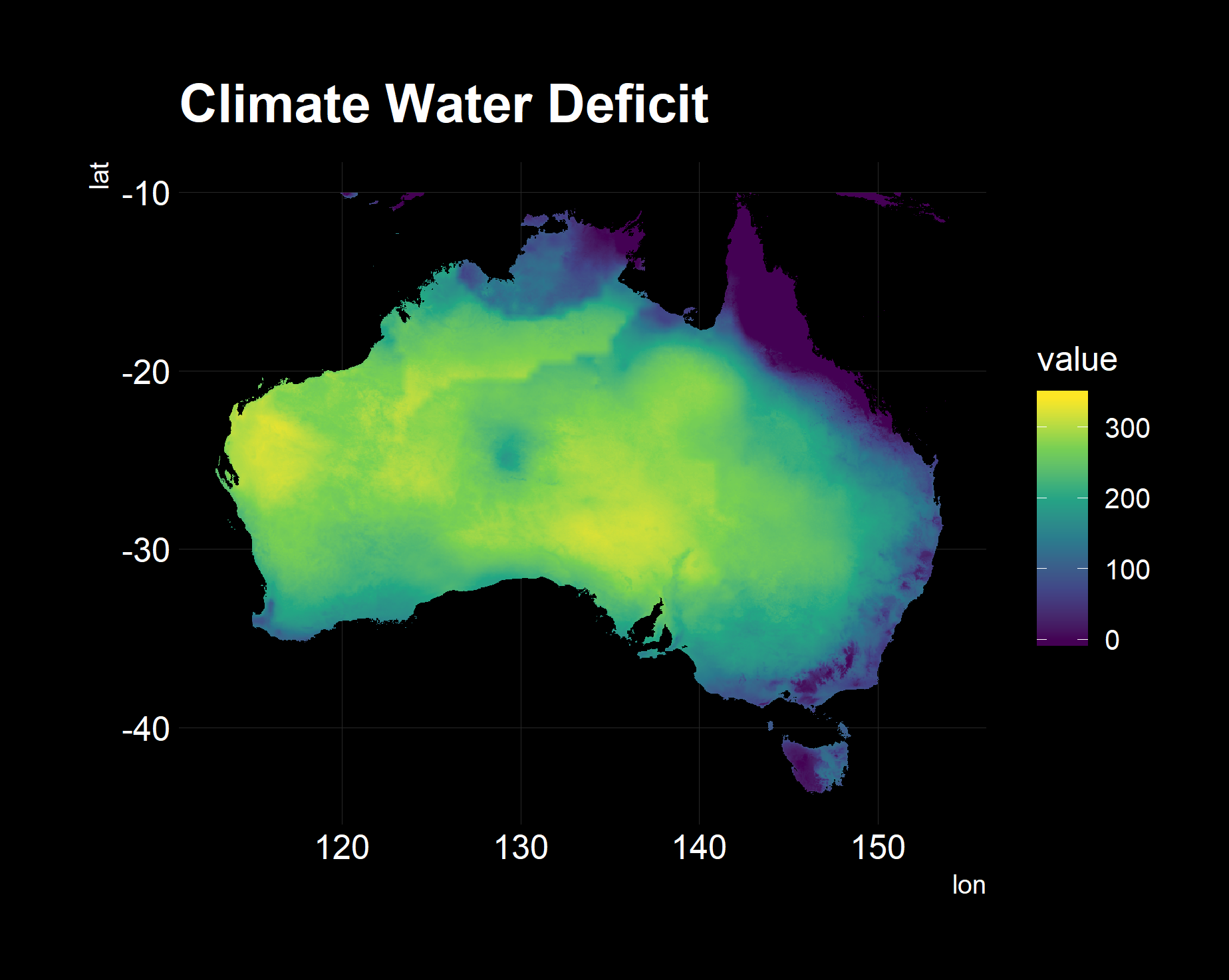
|def |Climate Water Deficit |
|pet |Potential evapotranspiration |
|ppt |Precipitation |
|q |Runoff |
|soil |Soil Moisture |
|srad |Downward surface shortwave radiation |
|swe |Snow water equivalent - at end of month |
|tmax |Max Temperature |
|tmin |Min Temperature |
|vap |Vapor pressure |
|ws |Wind speed |
|vpd |Vapor Pressure Deficit |
|PDSI |Palmer Drought Severity Index |The following code in 01 get ncdf data.R glues a string together and uses curl::curl_download to save the files into the respective folders. By naming the columns deliberately in df, we can exploit the argument matching capability of purrr::pwalk to get row-wise iteration over a dataframe.
require(pacman)
require(glue)
pacman::p_load(tidyverse, curl)
codes = read_csv("input/00 terraclimate codes/codes.csv", col_types = c("cc"))
year = 2018

url_builder = function(code, year){
  glue::glue("https://climate.northwestknowledge.net/TERRACLIMATE-DATA/TerraClimate_{str_to_upper(code)}_{year}.nc")
}

df = codes %>%
  mutate(url = map_chr(code, url_builder, year = year),
         destfile = glue::glue("input/01 climate ncdf/{year}_{code}.nc"))

df %>% select(url, destfile) %>% pwalk(curl_download)
I now had a folder full of .nc files with a grid of observations in three dimensions, latitude, longitude and time.
> files
 [1] "input/01 climate ncdf/2018_aet.nc"  "input/01 climate ncdf/2018_def.nc"
 [3] "input/01 climate ncdf/2018_PDSI.nc" "input/01 climate ncdf/2018_pet.nc"
 [5] "input/01 climate ncdf/2018_ppt.nc"  "input/01 climate ncdf/2018_q.nc"
 [7] "input/01 climate ncdf/2018_soil.nc" "input/01 climate ncdf/2018_srad.nc"
 [9] "input/01 climate ncdf/2018_swe.nc"  "input/01 climate ncdf/2018_tmax.nc"
[11] "input/01 climate ncdf/2018_tmin.nc" "input/01 climate ncdf/2018_vap.nc"
[13] "input/01 climate ncdf/2018_vpd.nc"  "input/01 climate ncdf/2018_ws.nc"
The approach I am taking here is derived from some trial and error, previous attempts to load and manipulate the NetCDF entirely in memory caused R to crash with my laptop’s 16GB of RAM.
In code for “02 ncdf to csv.R”, I nest a Monthly function inside a more substantial, per file function. Working backwards from the result I want, my data structure needs to have year, month, attribute, latitude, longitude and value. This data structure will be in a long format while I will eventually need it in a wide format for modelling.
This code subsets the NCDF via square brackets, into the third dimension, time. It also relies on the matrix having named rows and columns, which we will apply in the parent function.
Once this is done, I used pivot_longer to reshape the data frame from thousands of columns to five. I then convert the lat/lons into numerics and filter results to Australia and use data.table::setDT to change the type in place, i.e. no other objects are created in memory, very handy when working with large datasets and limited RAM. Finally some prayers to gods with gc() to free up memory, this is as superstitious as I get.
 per_month = function(selected_month, df, year){
    message(glue::glue("        {year} - {selected_month}"))

    # extract a month, pivot to long
    # Trying by month to fit all in mem
    df_monthly = df[, , selected_month] %>%
      as.data.frame(row.names = row.names(.)) %>%
      mutate(lon = row.names(.),
             attribute = attr_names,
             year = year,
             month = selected_month) %>%
      select(attribute, year, month, lon, everything()) %>%
      pivot_longer(cols = -(attribute:lon),
                   names_to = "lat",
                   values_to = "value") %>%
      mutate_at(vars(month:value), as.numeric) %>%
      filter(between(lat, -44, -10) & between(lon, 112, 154))

    # Convert to Data Table in memory so that we can use rbindlist to join quickly
    data.table::setDT(df_monthly)
    gc()
    df_monthly
  }
The next functions maps the per_month function to the time dimension of the NCDF matrix. By having a list of data.tables, I can use the blindingly fast data.table::rbindlist for row-based concatenation and writing the CSV back to disk.
per_file = function(file){

  year = str_extract(file,"[0-9]{4}") %>% as.numeric()
  message(glue::glue("opening {file}"))
  data = nc_open(file)
  attr_names = attributes(data$var)$names[1]
  dim_names = attributes(data$dim)$names
  message(glue::glue("    processing {str_pad(attr_names, 4, side = 'right')} - {year}"))

  df = ncvar_get(data, attr_names)
  lats = ncvar_get(data, dim_names[1])
  lons = ncvar_get(data, dim_names[2])

  # Assign names to dimensions so we can pivot long later on
  dimnames(df) = list(lon = lons, lat = lats)

  tidy_data = seq_len(dim(df)[3]) %>%
    map(per_month, df = df, year = year) %>%
    rbindlist() %>%
    arrange(month, lat, lon)

  fwrite(tidy_data, glue::glue("input/02 aus csv/{year}_{attr_names}_aus.csv"))
  message(glue::glue("    finished {str_pad(attr_names, 4, side = 'right')} - {year}"))
}
The third and final part of this post now looks at turning these long files into a single wide CSV. T
I wrote two, small helper functions in “03 long csvs to wide.R”. One for the common header data and a second to be mapped over all the CSVs. Having consistently used arrange in the previous code, I can simply column bind the single columns of results into a consistent, wide data.frame.
I also make using of R’s quasi-quotation to dynamically assign the column names in the “extract_attribute” function.
 extract_common = function(){
  "input/02 aus csv" %>%
    list.files(full.names = T, pattern = ".csv") %>%
    here::here() %>%
    magrittr::extract2(1) %>%
    fread() %>%
    select(year, month, lon, lat)
}

extract_attribute = function(file){
  all_data = file %>% fread()
  attribute = all_data$attribute[[1]]
  df = all_data %>% transmute(!! attribute := value)

  rm(all_data)
  gc()
  df
}
Bringing both pieces together is very straightforward. I also wrote a helper function to assist in verifying that the extract completed correctly.
df_common = extract_common()
df_attributes = files %>% map_dfc(extract_attribute)

df = df_common %>% bind_cols(df_attributes)
df %>% fwrite("input/03 wide csv/wide.csv")

attributes = df %>% select(-c(year:lat)) %>% colnames()

## Check Health of Attributes via plot
return_column_plot = function(col, df){
  # https://edwinth.github.io/blog/dplyr-recipes/
  col_enq = rlang::sym(col)

  title = fread("input/00 terraclimate codes/codes.csv") %>%
    filter(str_trim(code) == col) %>% pluck("description")

  df %>%
    dplyr::transmute(lon, lat, value = !!col_enq) %>%
    na.omit() %>%
    ggplot(aes(x = lon,
               y = lat,
               fill = value)) +
    geom_raster() +
    scale_fill_viridis_c() +
    coord_equal() +
    labs(title = title) +
    hrbrthemes::theme_ipsum_rc() +
    theme(
      panel.background = element_rect(fill = "black"),
      plot.background = element_rect(fill = "black"),
      legend.background = element_rect(fill = "black"),
      text = element_text(colour = "white"),
      axis.text = element_text(colour = "white"),
      panel.grid.major.x = element_line(colour = rgb(40, 40, 40, maxColorValue = 255)),
      panel.grid.major.y = element_line(colour = rgb(40, 40, 40, maxColorValue = 255))
    ) +
    ggthemr::no_minor_gridlines()

  ggsave(
    glue::glue("plot/attributes/{col}.png"),
    width = 5,
    height = 5,
    units = "cm",
    dpi = 320,
    scale = 3
  )
}

attributes %>% walk(return_column_plot, df = df %>%
                      filter(year == max(year)) %>%
                      mutate_at(vars(aet:ws), as.numeric))
The following are graphs used in spot-checking the validity. All looks well!
This completes the climate component of the data collection stage. Further detail to come in subsequent posts.